Surface wave identification

↑ Click on “Open in Colab” to execute this notebook live on Google Colaboratory.

Getting Started

First, we need to mount the Google Drive so we can access the Distributed Acoustic Sensing data stored in it. After execution, the following script will provide a link. Open the link and follow the instructions to get the one-time password. If you have several Google accounts logged on your computer, make sure you use the one the DAS data were shared with.

Some of the data used in this work are proprietary data and may be shared under specific circumstances. Please contact the corresponding author, Vincent Dumont if you would like to request access to the data or have any questions regarding this project.

Upon authorization to share the data, a link to a shared Google Drive folder will be send to you. After clicking on the link, the shared folder (called DAS_data ) will be listed under the Shared with me section of your Google Drive, you can then do a right click on that folder and click Add shortcut to Drive , this will add the folder to your My Drive repository.

Finally, executing the following cell will mount your Google Drive to this instance of Google Colab and give you access to the data:

import os
from google.colab import drive
drive.mount('/content/drive')

Mounted at /content/drive

General settings

import matplotlib.pyplot as plt
plt.style.use('seaborn')
plt.rc('font', size=15)
plt.rc('axes', labelsize=15)
plt.rc('legend', fontsize=15)
plt.rc('xtick', labelsize=15)
plt.rc('ytick', labelsize=15)

data_path = '/content/drive/MyDrive/DAS_data/'

Software installation

All the figures in this work can be reproduced using our MLDAS software, which can be loaded as follows:

%%capture
!git clone https://gitlab.com/ml4science/mldas
!pip install -r mldas/requirements.txt
!ln -s /content/mldas/mldas $(python -c "import pip; print(pip.__path__[0].rstrip('/pip'))")/

Fig. 2: All channels, one minute

import h5py, numpy
f = h5py.File(data_path+'fullLine_1min_180108163831.mat','r')
data = f[f.get('dsi/dat')[0,0]]
data = abs(numpy.array(data))
data[numpy.where(data==0)] = 1

import matplotlib.pyplot as plt
from matplotlib.colors import LogNorm
fig,ax = plt.subplots(figsize=(9,6))
ax.grid(False)
plt.imshow(data.T,extent=[0,data.shape[0],data.shape[1]/500,0],cmap='inferno',aspect='auto',norm=LogNorm())
ax.axvline(4650,color='cyan',lw=3)
ax.axvline(4850,color='cyan',lw=3)
ax.axvline(5500,color='yellow',lw=3)
ax.axvline(6000,color='yellow',lw=3)
ax.xaxis.set_ticks_position('top')
ax.xaxis.set_label_position('top')
plt.xlabel('Channels',labelpad=10)
plt.ylabel('Time [second]')
plt.colorbar(pad=0.02,orientation="horizontal").set_label('DAS units (proportional to strain rate)')
plt.tight_layout()
plt.savefig('abs_data.png')
plt.show()
plt.close()

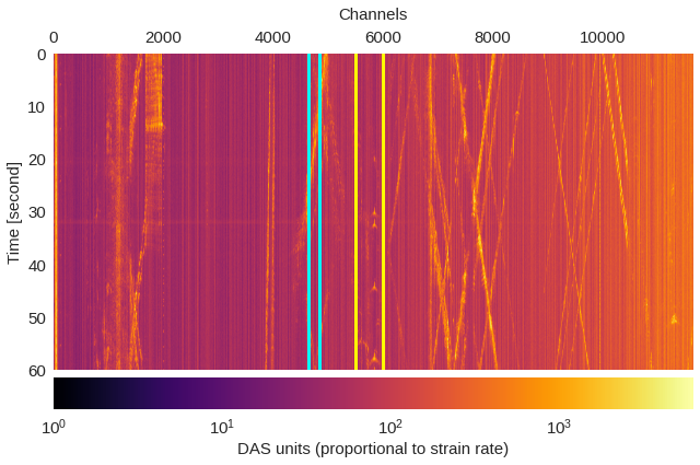
Fig. 3: Example regions

import h5py, numpy
# First region
f = h5py.File(data_path+'30min_files_Train/Dsi_30min_170730203007_170730210007_ch5500_6000_NS.mat','r')
data1 = numpy.array(f[f.get('dsi30/dat')[0,0]][2:202,467553:468153])
f.close()
# Second region
f = h5py.File(data_path+'1min_ch4650_4850/180104/westSac_180104001631_ch4650_4850.mat','r')
data2 = numpy.array(f[f.get('variable/dat')[0,0]][0:200,14000:14600])
f.close()

import matplotlib.pyplot as plt
from mpl_toolkits.axes_grid1.axes_divider import make_axes_locatable
# Initialize figure
fig,ax = plt.subplots(1,2,figsize=(18,5.5))
# Plot coherent surface wave patterns
im = ax[0].imshow(data1,extent=[0,data1.shape[1],200,0],cmap='seismic',aspect='auto',vmin=-1000,vmax=1000,interpolation='bicubic')
ax[0].xaxis.set_ticks_position('top')
ax[0].xaxis.set_label_position('top')
ax[0].set_xlabel('Samples',labelpad=10)
ax[0].set_ylabel('Channels')
# Display colorbar
divider = make_axes_locatable(ax[0])
cax = divider.append_axes('bottom', size='5%', pad=0.05)
plt.colorbar(im, pad=0.02, cax=cax, orientation='horizontal').set_label('Raw measurement amplitude')
# Plot non-coherent signals
im = ax[1].imshow(data2,extent=[0,data2.shape[1],200,0],cmap='seismic',aspect='auto',vmin=-1000,vmax=1000,interpolation='bicubic')
ax[1].xaxis.set_ticks_position('top')
ax[1].xaxis.set_label_position('top')
ax[1].set_xlabel('Samples',labelpad=10)
ax[1].set_ylabel('Channels')
# Display colorbar
divider = make_axes_locatable(ax[1])
cax = divider.append_axes('bottom', size='5%', pad=0.05)
plt.colorbar(im, pad=0.02, cax=cax, orientation='horizontal').set_label('Raw measurement amplitude')
# Save and show figure
plt.tight_layout()
plt.savefig('raw_data.pdf')
plt.show()
plt.close()

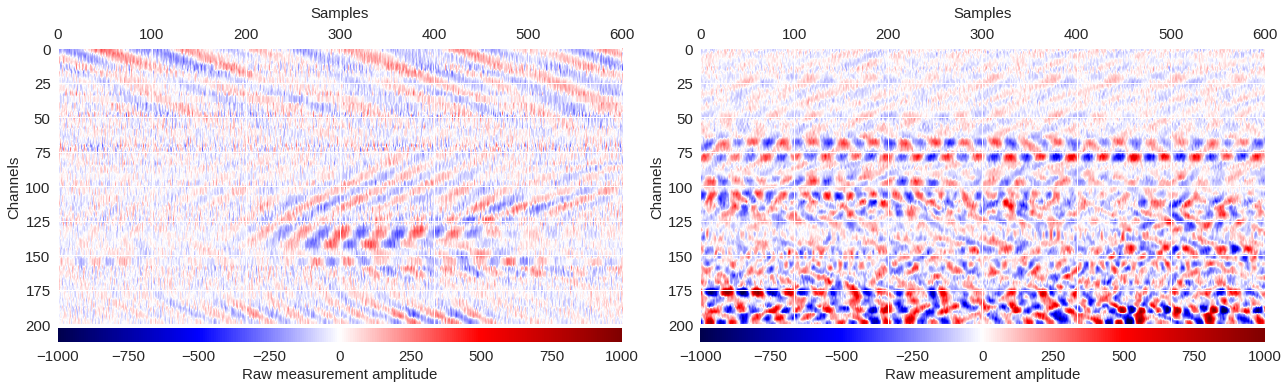
Fig. 4: Raw data distribution

Here, we will look at the distributions of the raw strain measurements and fit them using both single and double gaussian fitting.

import h5py
import numpy
f = h5py.File(data_path+'1min_ch4650_4850/180103/westSac_180103010131_ch4650_4850.mat','r')
data = numpy.array(f[f.get('variable/dat')[0,0]])
f.close()

As one can see below, a double gaussian provides a much better fit to the data. The two gaussians could be interpreted as one fitting the white noise data (narrow gaussian) and the other fitting the broader distribution from surface wave regions.

import matplotlib.pyplot as plt
from mldas.utils import gaussian_fit
fig,ax = plt.subplots(2,1,figsize=(9,8),sharey=True,sharex=True)
for i,order in enumerate([1,2]):
  hist = ax[i].hist(data.reshape(numpy.prod(data.shape)),bins=400,range=[-1000,1000],color='white',histtype='stepfilled',edgecolor='black',lw=0.5)
  # Fit double gaussian
  x = numpy.array([0.5 * (hist[1][i] + hist[1][i+1]) for i in range(len(hist[1])-1)])
  y = hist[0]
  x, y, chisq, aic, popt = gaussian_fit(x,y,order)
  if order==1:
    ax[i].plot(x, y[0], lw=2,label='Single-gaussian fit\n$\chi^2_\mathrm{red}=$%.1e / $\mathrm{AIC}=%i$\n$\mu=%.2f, \sigma=%.3f$'%(chisq,aic,popt[1],abs(popt[2])))
  if order==2:
    ax[i].plot(x, y[0], lw=2,label='Double-gaussian fit\n$\chi^2_\mathrm{red}=$%.1e / $\mathrm{AIC}=%i$'%(chisq,aic))
    # Plot first gaussian
    # y = gauss_single(x, *popt[:3])
    ax[i].plot(x, y[1], lw=2,label=r'$\mu=%.2f, \sigma=%.3f$'%(popt[1],abs(popt[2])))
    # Plot second gaussian
    # y = gauss_single(x, *popt[3:])
    ax[i].plot(x, y[2], lw=2,label=r'$\mu=%.2f, \sigma=%.3f$'%(popt[4],abs(popt[5])))
    ax[i].ticklabel_format(axis="y", style="sci", scilimits=(0,0))
  ax[i].set_xlim(-1000,1000)
  ax[i].legend(loc='upper left')
  ax[i].set_ylabel('Density')
plt.xlabel('Raw measurement amplitude')
plt.tight_layout()
plt.savefig('distribution.pdf')

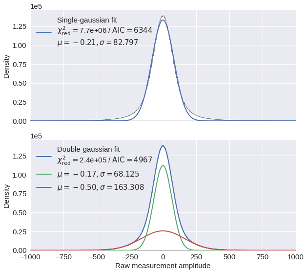
Fig. 5: Frequency content

data_samples = [[201, 384672, data_path+'30min_files_Train/Dsi_30min_170730023007_170730030007_ch5500_6000_NS.mat'],
                [193, 921372, data_path+'30min_files_Train/Dsi_30min_170730023007_170730030007_ch5500_6000_NS.mat'],
                [  0,  15000, data_path+'1min_ch4650_4850/180104/westSac_180104001631_ch4650_4850.mat'            ],
                [170, 685516, data_path+'30min_files_Train/Dsi_30min_170730023007_170730030007_ch5500_6000_NS.mat']]

data = []
for i,j,data_sample in data_samples:
  key = 'dsi30' if '30min' in data_sample else 'variable'
  f = h5py.File(data_sample,'r')
  img = f[f.get(key+'/dat')[0,0]][i:i+200,j:j+200]
  data.append(img)
  f.close()

import matplotlib.pyplot as plt
from matplotlib.colors import LogNorm
from matplotlib.offsetbox import AnchoredText
from mldas.utils import freq_content
plt.rc('font', size=12)
plt.rc('axes', labelsize=12)
plt.rc('legend', fontsize=12)
plt.rc('xtick', labelsize=12)
plt.rc('ytick', labelsize=12)
fig,ax = plt.subplots(4,4,figsize=(12,12))
for n,img in enumerate(data):
  ffts, freqs, avg_fft = freq_content(img,200,500)
  img_max = abs(img).max()
  # Show larger image
  ax[0][n].imshow(img,cmap='seismic',extent=[0,200,200,0],vmin=-img_max,vmax=img_max,interpolation='bicubic')
  ax[0][n].set_xlabel('Sample')
  if n==0: ax[0][n].set_ylabel('Channel')
  # Plotting data distribution
  ax[1][n].hist(img.reshape(numpy.prod(img.shape)),bins=50)
  at = AnchoredText('$\sigma=%i$'%numpy.std(img),prop=dict(size=12),loc='upper left')
  ax[1][n].add_artist(at)
  ax[1][n].set_xlabel('Strain Measurement')
  if n==0: ax[1][n].set_ylabel('Density')
  # D2 and plot FFT for each channel
  ax[2][n].imshow(ffts,extent=[0,500//2,img.shape[0],0],aspect='auto',norm=LogNorm(vmin=ffts.min(),vmax=ffts.max()),cmap='jet')
  ax[2][n].set_xlabel('Frequency (Hz)')
  if n==0: ax[2][n].set_ylabel('Channels')\
  # Plot average amplitude for each frequency
  ax[3][n].plot(freqs,avg_fft)
  ax[3][n].set_xlabel('Frequency (Hz)')
  ax[3][n].set_xlim(0,500//2)
  ax[3][n].axvline(40,ls='--',color='black',lw=1.3)
  ax[3][n].set_ylabel('Average Spectral Amplitude')
plt.tight_layout(h_pad=0,w_pad=0)
plt.savefig('signal_types.pdf')
plt.show()

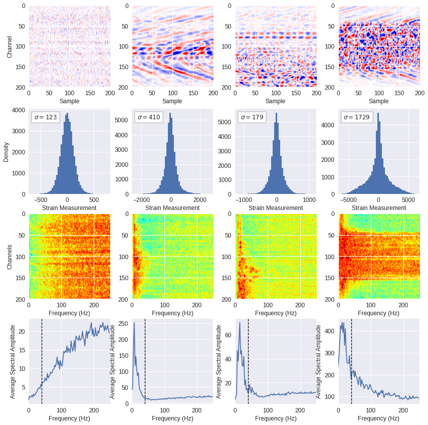
Fig. 6: Training images

Training images were selected within the 30-minute DAS data files, the following will shuffle the 146 data files containing 30 minutes of DAS data, 43 of those files contain a train trace, the remaining 103 data files do not contain train trace.

import glob,numpy,random
filelist = glob.glob(data_path+'30min_files_*Train/*mat')
random.shuffle(filelist)

The following two commands will create the datasets within a structure readable by the PyTorch library. The first function ( find_target ) will read through the entire file list loaded above and randomly identify patches of data that match either noise or waves selection criteria. The second function ( create_set ) will gather all noise and waves images recorded across all files and create train, test and validation dataset folders with 70/15/15 percent of images per label on each folder respectively.

from mldas.datasets import generate
generate.find_target(filelist) # Can take a long time process
generate.create_set('/content/Dsi_*',imax=174000)

The creation of the datasets can take some time to process. Therefore, for timing purposes, we will use in this notebook a pre-created dataset of 174,000 images which we can extract locally as follows:

import tarfile
tar = tarfile.open(data_path+'train_data.tar.gz')
tar.extractall()
tar.close()

The following snippet will display 25 examples of waves images and 25 examples of noise images among the loaded dataset.

import random,glob
import matplotlib.pyplot as plt
plt.style.use('seaborn')
plt.figure(figsize=(15,7),dpi=80)
for label,offset in [['waves',0],['noise',6]]:
  dataset = random.sample(glob.glob('/content/train/%s/*.jpg'%label),25)
  for i,fname in enumerate(dataset):
    ax = plt.subplot(5,11,(i+1)-5*(i//5)+11*(i//5)+offset)
    ax.axis('off')
    ax.imshow(plt.imread(fname),cmap='binary')
plt.tight_layout()
plt.savefig('train_data.pdf')
plt.show()

!rm -rf /content/test /content/train /content/validation

Fig. 7: Latent representation

The autoencoder was explored on 20,000 images with 50x50 dimensions. A pre-created dataset can be loaded as follows:

import tarfile
tar = tarfile.open(data_path+'train_data_for_vae.tar.gz')
tar.extractall()
tar.close()

The training dataset can be easily loaded in PyTorch using the ImageFolder class. We use a batch size of 100 to prepare the data loader:

import torch
from torchvision import transforms, datasets
mytransforms = transforms.Compose([transforms.Grayscale(),transforms.ToTensor()])
trainset = datasets.ImageFolder(root='/content/train',transform=mytransforms)
train_loader = torch.utils.data.DataLoader(trainset,batch_size=100,shuffle=True)

The shallow variational autoencoder will be trained for 10 epochs, the model will be saved at the end of each epoch so we can visualize afterwards how the latent representation evolves across training epochs.

from mldas.trainers import vae
trainer = vae.VAETrainer()
losses, models = trainer.train_model(train_loader,epochs=10)

==> Epoch 1/10 | Duration: 26.2519 seconds | Loss: 1734.189
==> Epoch 2/10 | Duration: 18.2687 seconds | Loss: 1733.369
==> Epoch 3/10 | Duration: 18.1504 seconds | Loss: 1732.912
==> Epoch 4/10 | Duration: 19.6028 seconds | Loss: 1732.708
==> Epoch 5/10 | Duration: 19.6968 seconds | Loss: 1732.474
==> Epoch 6/10 | Duration: 20.2220 seconds | Loss: 1732.129
==> Epoch 7/10 | Duration: 19.7561 seconds | Loss: 1731.955
==> Epoch 8/10 | Duration: 20.4259 seconds | Loss: 1731.850
==> Epoch 9/10 | Duration: 20.2006 seconds | Loss: 1731.716
==> Epoch 10/10 | Duration: 20.9147 seconds | Loss: 1731.613
Full loop over 10 epochs processed in 203.4965 seconds

The latent representation is shown below for the training set with a color scheme reflecting the label with noise images characterized by the color blue (value of 0) and surface wave images by the color pink (value of 1).

The figure may slightly difer from the published figure because of the intrinsic stochasticity of the training which makes the outcomes look different.

import matplotlib.pyplot as plt
fig, ax = plt.subplots(3,2,figsize=(10,12),sharex=True,sharey=True)
axs = ax.flatten()
for n,ax in enumerate(axs):
  model_epoch = models[n]
  model_epoch.eval()
  for batch_idx, (data,target) in enumerate(train_loader):
    data = data.float()
    z, recon_batch, mu, logvar = model_epoch(data.view(-1,numpy.prod(data.shape[-2:])))
    z = z.data.cpu().numpy()
    ax.scatter(z[:,0],z[:,1],s=10,c=target,cmap='cool',alpha=0.5)
  ax.set_title('Epoch %i'%(n+1),fontsize=15)
  if n>=4: ax.set_xlabel('Latent variable 1')
  if n%2==0: ax.set_ylabel('Latent variable 2')
plt.tight_layout()
plt.savefig('clustering.pdf')
plt.show()

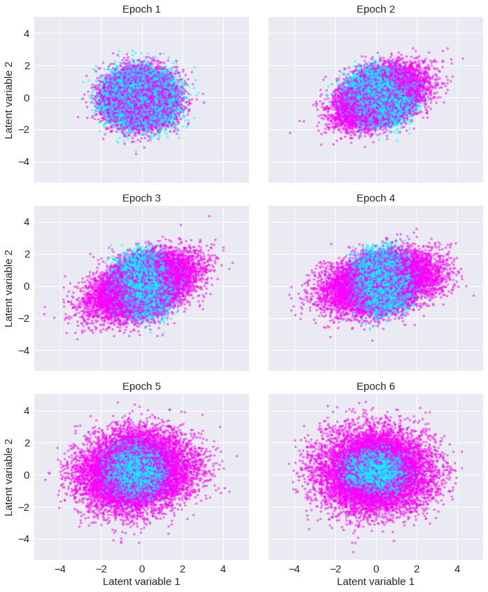
Fig. 8: Distribution performance

import tarfile
tar = tarfile.open(data_path+'all_jobs.tar.gz')
tar.extractall()
tar.close()

import glob
import pandas as pd
results_files = glob.glob('/content/all_jobs/multiclass/2-neuron/1-channel/gpu-n*-ds10-bs256-ep50-dp14-lr0.01/results.txt')
results = [pd.read_csv(f, delim_whitespace=True) for f in results_files]
results = pd.concat(results, ignore_index=True)
results = results.sort_values('ranks')[:-1]
ranks = results.ranks.values
rates = results.train_rate.values
results

	train_rate	inference_rate	ranks	hardware	version	backend	model
1	586.452987	999.830839	2	gpu	v1.5.0	nccl	resnet
0	1076.182053	1837.489459	4	gpu	v1.5.0	nccl	resnet
3	1845.965617	3158.509798	8	gpu	v1.5.0	nccl	resnet
5	1445.493348	2305.639525	12	gpu	v1.5.0	nccl	resnet
2	3316.106960	6356.857673	16	gpu	v1.5.0	nccl	resnet

plt.style.use('seaborn')
plt.rc('font', size=17)
plt.rc('axes', labelsize=17)
plt.rc('legend', fontsize=17)
plt.rc('xtick', labelsize=17)
plt.rc('ytick', labelsize=17)
fig, (ax0, ax1) = plt.subplots(nrows=1, ncols=2, figsize=(14, 6), sharex=True)
# Compute ideal scaling relative to lowest rank
ideal_rates = rates[0] * ranks / ranks[0]
# Plot throughput scaling
ax0.plot(ranks, rates, '.-', ms=15, label='measured')
ax0.plot(ranks, ideal_rates, '--', label='ideal')
ax0.set_xlabel('Number of GPUs')
ax0.set_ylabel('Training throughput [samples/s]')
ax0.set_ylim(bottom=0)
# ax0.grid()
ax0.legend(loc=0)
# Plot the fraction of ideal scaling
ax1.plot(ranks, rates / ideal_rates, '.-', ms=15)
ax1.set_xlabel('Number of GPUs')
ax1.set_ylabel('Fraction of ideal scaling')
# ax1.grid()
ax1.set_ylim(bottom=0)
plt.tight_layout()
plt.savefig('scaling.pdf')
plt.show()

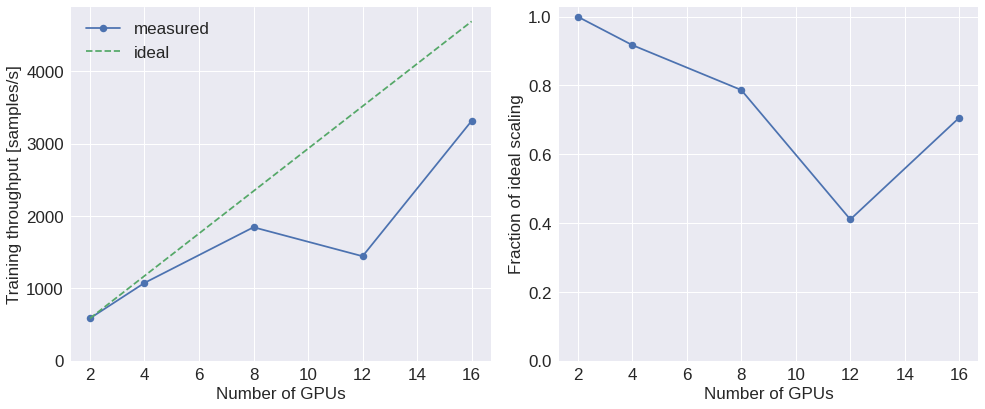
Fig. 9: Best model

import numpy
out = open('/content/all_jobs/multiclass/2-neuron/3-channel/gpu-n8-ds1-bs128-ep51-dp14-lr0.001/out_0.log','r')
train_loss, train_acc, valid_loss, valid_acc = [], [], [], []
for line in out:
  if 'Training' in line :
    train_loss.append(float(line.split()[-4]))
    train_acc.append(float(line.split()[-1]))
  if 'Validation' in line:
    valid_loss.append(float(line.split()[-4]))
    valid_acc.append(float(line.split()[-1]))
out.close()

import matplotlib.pyplot as plt
plt.figure(figsize=(10,6),dpi=80)
plt.plot(train_acc,label='Training')
plt.plot(valid_acc,label='Validation')
plt.xlabel('Epochs')
plt.ylabel('Accuracy')
plt.ylim(ymax=100)
plt.legend(loc='best')
plt.tight_layout()
plt.savefig('best_model.pdf')
plt.show()

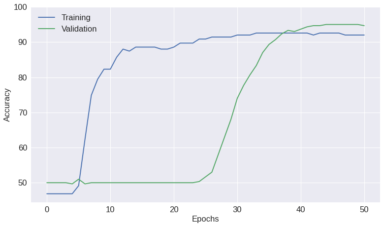
Fig. 10: Probability time series

We can now use trained model to do inference and estimate the probability of usable seismic energy at every time and space locations throughout the entire fiber and the whole 10 days of recorded data. Given the large number of DAS data files to process during inference (1-minute data during 10 days or 14,400 files in total), we executed it in parallel using the mpi4py library on the Cori supercomputer. The MLDAS software can execute the inference after being provided with a list of user-input parameters which can be included within a yaml file such as follows:

# img_size: 200
# channel_stride: 200
# sample_stride: 200
# num_channels: 3
# num_classes: 2
# model_file: trained_model.pth.tar
# data_path: 1min_ch4650_4850/
# model_type: resnet
# multilabel: False
# compact: False
# depth: 14

The following SLURM script will execute the inference on Cori across 96 CPU processes (3 full CPU nodes):

#!/bin/bash
#SBATCH -N 3
#SBATCH -q regular
#SBATCH -t 05:00:00
#SBATCH -C haswell
#SBATCH -J prob-multiproc
#SBATCH -o logs/%x-%j.out
module load pytorch/v1.6.0
srun -n 96 -c 2 python $HOME/mldas/mldas/assess.py probmap -c $HOME/mldas/configs/assess.yaml -o $SCRATCH/probmaps --mpi

This will call the das_assess.py script which will execute internally the mldas.sh script which will itself trigger the mldas.explore.production.probmap function. Below we extract pre-saved probability map from all the 1-minute DAS data files from channels 4650 to 4850.

import tarfile
tar = tarfile.open(data_path+'probability_maps.tar.gz')
tar.extractall()
tar.close()

Below we calculate the mean of each 1-minute data file:

import glob,numpy,re,datetime
file_list = glob.glob('/content/probmaps/*.txt')
results = numpy.empty((0,2))
for fname in sorted(file_list):
  date = [int(i) for i in re.findall('..?',fname.split('_')[1])]
  date = datetime.datetime(2000+date[0],*date[1:])+datetime.timedelta(hours=-8)
  prob = numpy.mean(numpy.loadtxt(fname))
  results = numpy.vstack((results,[date,prob]))
print(results.shape)

(14399, 2)

A smoother version of the data can be obtained by resampling the data an applying a Gaussian filter:

import numpy
from scipy import signal,ndimage
y = signal.resample(results[:,1],len(results[:,1])//10)
b = signal.gaussian(39, 10)
y = ndimage.filters.convolve1d(y, b/b.sum())
x = results[::len(results)//len(y),0][:-1]
print(len(x),len(y))

1439 1439

import matplotlib.pyplot as plt
import matplotlib.dates as mdates
fig,ax = plt.subplots(figsize=(14,6),dpi=100)
ax.plot(results[:,0],results[:,1])
ax.plot(x,y,color='yellow')
ax.xaxis.set_major_formatter(mdates.DateFormatter('%A\n%Y-%m-%d'))
ax.set_ylabel('Surface wave probability')
ax.set_xlim(results[0,0],results[-1,0])
plt.tight_layout()
plt.savefig('prob_time_series.pdf')
plt.show()

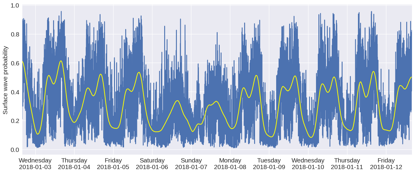
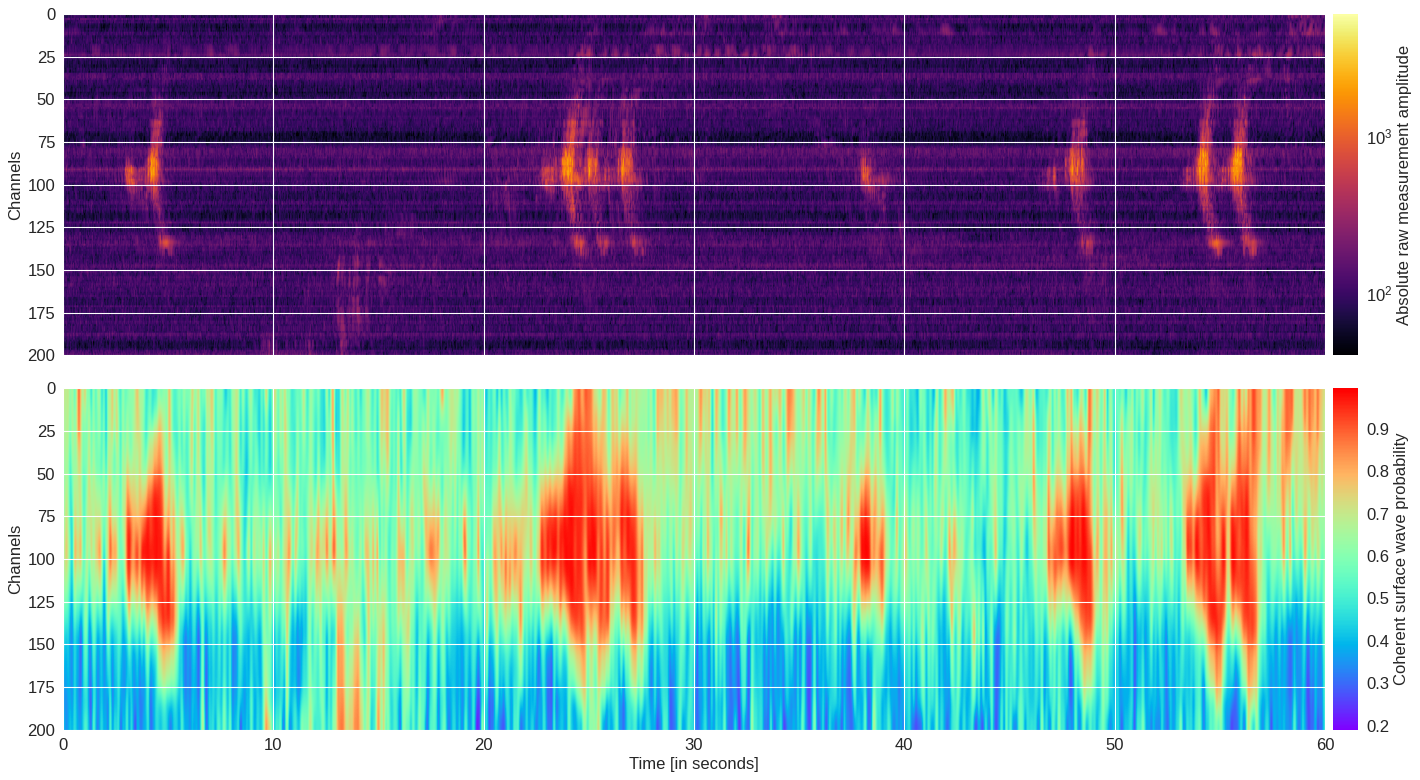
Fig. 11: Probability map

import h5py,numpy,torch
from mldas.models.resnet import ResNet
from mldas.explore import extract_prob_map
f = h5py.File(data_path+'30min_files_NoTrain/Dsi_30min_170803233007_170804000007_ch5500_6000.mat','r')
data = numpy.array(f[f.get('data/dat')[0,0]][300:500,:30000])
model = ResNet(depth=8,num_classes=2,num_channels=3)
model.load_state_dict(torch.load(data_path+'model39.pt'))
probmap = extract_prob_map(data,model,img_size=50,channel_stride=10,sample_stride=50,rgb=True,colormap='gist_earth')
data = abs(data)
data[numpy.where(data==0)] = 1

import matplotlib.pyplot as plt
from matplotlib.colors import LogNorm
from mpl_toolkits.axes_grid1.axes_divider import make_axes_locatable
fig,(ax0,ax1) = plt.subplots(2,1,figsize=(18,10),dpi=80,sharex=True)
im = ax0.imshow(data,aspect='auto',extent=[0,60,200,0],cmap='inferno',norm=LogNorm(vmin=40))
divider = make_axes_locatable(ax0)
cax = divider.append_axes('right', size='2%', pad=0.1)
plt.colorbar(im, pad=0.02, cax=cax, orientation='vertical').set_label('Absolute raw measurement amplitude')
ax0.set_ylabel('Channels')
im = ax1.imshow(probmap,aspect='auto',extent=[0,60,200,0],cmap='rainbow',interpolation='bicubic')
divider = make_axes_locatable(ax1)
cax = divider.append_axes('right', size='2%', pad=0.1)
plt.colorbar(im, pad=0.02, cax=cax, orientation='vertical').set_label('Coherent surface wave probability')
ax1.set_ylabel('Channels')
ax1.set_xlabel('Time [in seconds]')
plt.tight_layout()
plt.savefig('probmap.pdf')
plt.show()