Image segmentation ¶

In this notebook, we show how to apply an image segmentation method to the DAS data and explore different approaches. The goal of image segmentation algorithms is to group nearby pixels with common characteristics.

[ ]:

           from google.colab import drive
drive.mount('/content/drive')

Segmentation model ¶

Trained supervised models ¶

PyTorch already provides several pre-trained segmentation model. Here, we will evaluate two pre-trained model from PyTorch, the Fully Convolutional Network (FCN) and the DeepLab v3 model. This page , and the notebook therein, provide a very good introduction in how to use those models. Both models can be easily loaded using the torchvision library as follows:

[2]:

             %%capture
from torchvision import models
fcn = models.segmentation.fcn_resnet101(pretrained=True).eval()
dlab = models.segmentation.deeplabv3_resnet101(pretrained=True).eval()

            

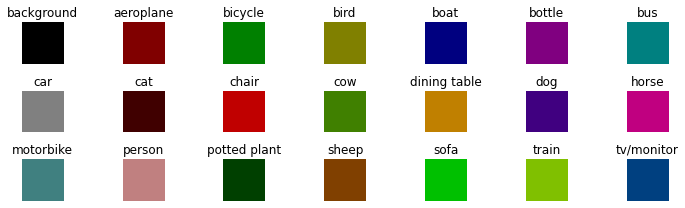
Since this is a supervised approach, image segmentation masks were created that contain the target label for every pixel in the training images. Those masks will be used to train the model. Below we show which color is associated to each label in the dataset.

[ ]:

             import numpy
import matplotlib.pyplot as plt
labels = numpy.array([[(0, 0, 0),'background'],[(128, 0, 0), 'aeroplane'],[(0, 128, 0), 'bicycle'],[(128, 128, 0), 'bird'],
                      [(0, 0, 128), 'boat'],[(128, 0, 128), 'bottle'],[(0, 128, 128),'bus'], [(128, 128, 128),'car'],
                      [(64, 0, 0),'cat'], [(192, 0, 0),'chair'], [(64, 128, 0),'cow'],[(192, 128, 0),'dining table'],
                      [(64, 0, 128),'dog'], [(192, 0, 128),'horse'], [(64, 128, 128),'motorbike'], [(192, 128, 128),'person'],
                      [(0, 64, 0),'potted plant'], [(128, 64, 0),'sheep'], [(0, 192, 0),'sofa'], [(128, 192, 0),'train'],
                      [(0, 64, 128),'tv/monitor']])
label_colors = numpy.zeros((len(labels),3),dtype=numpy.uint8)
fig, ax = plt.subplots(3,7,figsize=(10,3))
for i,(color,label) in enumerate(labels):
  label_colors[i] = list(color)
  ax[i//7][i-7*(i//7)].imshow(label_colors[i].reshape(1,1,3))
  ax[i//7][i-7*(i//7)].set_title(label)
  ax[i//7][i-7*(i//7)].axis('off')
plt.tight_layout()
plt.show()

            

The function below will convert the 2D image to an RGB image where each label is mapped to its corresponding color.

[ ]:

             import numpy
def decode_segmap(image, label_colors, nc=21):
  """
  Converting segmentation image into label mapping
  """
  r = numpy.zeros_like(image).astype(numpy.uint8)
  g = numpy.zeros_like(image).astype(numpy.uint8)
  b = numpy.zeros_like(image).astype(numpy.uint8)
  for l in range(0, nc):
    idx = image == l
    r[idx] = label_colors[l, 0]
    g[idx] = label_colors[l, 1]
    b[idx] = label_colors[l, 2]
  rgb = numpy.stack([r, g, b], axis=2)
  return rgb

            

[ ]:

             import torch
import matplotlib.pyplot as plt
import torchvision.transforms as T
from PIL import Image
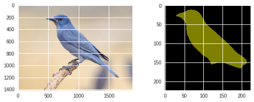
def segment(net, path, label_colors):
  img = Image.open(path)
  # Comment the Resize and CenterCrop for better inference results
  trf = T.Compose([T.Resize(256),
                   T.CenterCrop(224),
                   T.ToTensor(),
                   T.Normalize(mean = [0.485, 0.456, 0.406],
                               std = [0.229, 0.224, 0.225])])
  inp = trf(img).unsqueeze(0)
  out = net(inp)['out']
  om = torch.argmax(out.squeeze(), dim=0).detach().cpu().numpy()
  rgb = decode_segmap(om, label_colors)
  plt.style.use('seaborn')
  fig,(ax1,ax2) = plt.subplots(1,2,figsize=(8,3))
  ax1.imshow(img)
  ax2.imshow(rgb)
  plt.tight_layout()
  plt.show()

            

[ ]:

             !wget -nv https://static.independent.co.uk/s3fs-public/thumbnails/image/2018/04/10/19/pinyon-jay-bird.jpg -O bird.png
segment(fcn, './bird.png', label_colors)
segment(dlab, './bird.png', label_colors)

            

2020-09-05 05:29:35 URL:https://static.independent.co.uk/s3fs-public/thumbnails/image/2018/04/10/19/pinyon-jay-bird.jpg [182965/182965] -> "bird.png" [1]

../_images/segmentation_segment_10_1.png

../_images/segmentation_segment_10_2.png

Untrained supervised model ¶

[ ]:

             %%capture
from torchvision import models
fcn = models.segmentation.fcn_resnet101(pretrained=False)
dlab = models.segmentation.deeplabv3_resnet101(pretrained=False)

            

Unsupervised model ¶

For this first implementation, we used a Convolutional Neural Network (CNN) model from this work .

[3]:

             import torch.nn as nn
class Kanezaki(nn.Module):
    def __init__(self,input_dim):
        super(Kanezaki, self).__init__()
        self.conv1 = nn.Conv2d(input_dim, args.nChannel, kernel_size=3, stride=1, padding=1 )
        self.bn1 = nn.BatchNorm2d(args.nChannel)
        self.conv2 = nn.ModuleList()
        self.bn2 = nn.ModuleList()
        for i in range(args.nConv-1):
            self.conv2.append( nn.Conv2d(args.nChannel, args.nChannel, kernel_size=3, stride=1, padding=1 ) )
            self.bn2.append( nn.BatchNorm2d(args.nChannel) )
        self.conv3 = nn.Conv2d(args.nChannel, args.nChannel, kernel_size=1, stride=1, padding=0 )
        self.bn3 = nn.BatchNorm2d(args.nChannel)

    def forward(self, x):
        x = self.conv1(x)
        x = F.relu( x )
        x = self.bn1(x)
        for i in range(args.nConv-1):
            x = self.conv2[i](x)
            x = F.relu( x )
            x = self.bn2[i](x)
        x = self.conv3(x)
        x = self.bn3(x)
        return x

            

Training a segmentation model ¶

[15]:

            import argparse
parser = argparse.ArgumentParser(description='PyTorch Unsupervised Segmentation')
# Original values: nChannel 100, maxIter 1000, minLabels 3, lr 0.1, nConv 2
parser.add_argument('--nChannel',        metavar='N',    default=100,   type=int,   help='number of channels')
parser.add_argument('--maxIter',         metavar='T',    default=100,   type=int,   help='number of maximum iterations')
parser.add_argument('--minLabels',       metavar='minL', default=3,     type=int,   help='minimum number of labels')
parser.add_argument('--lr',              metavar='LR',   default=0.1,   type=float, help='learning rate')
parser.add_argument('--nConv',           metavar='M',    default=2,     type=int,   help='number of convolutional layers')
parser.add_argument('--num_superpixels', metavar='K',    default=10000, type=int,   help='number of superpixels')
parser.add_argument('--compactness',     metavar='C',    default=100,   type=float, help='compactness of superpixels')
# args = parser.parse_args()
args = parser.parse_known_args()[0]

           

Simple Linear Iterative Clustering ¶

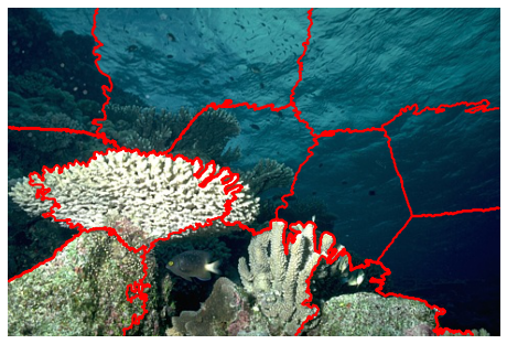
As described in this page , the Simple Linear Iterative Clustering (or SLIC) algorithm generates superpixels by clustering pixels based on their color similarity and proximity in the image plane. One can use the slic class from the skimage package to do the clustering.

[68]:

             from skimage import segmentation
labels = segmentation.slic(im, compactness=50, n_segments=16)
print('Segmentation image:\n',labels)
u_labels = numpy.unique(labels)
print(len(u_labels),'total number of labels:\n',u_labels)

            

Segmentation image:
 [[ 0  0  0 ...  4  4  4]
 [ 0  0  0 ...  4  4  4]
 [ 0  0  0 ...  4  4  4]
 ...
 [13 13 13 ... 10 10 10]
 [13 13 13 ... 10 10 10]
 [13 13 13 ... 10 10 10]]
15 total number of labels:
 [ 0  1  2  3  4  5  6  7  8  9 10 11 12 13 14]

Below we show what the clustering looks like by overplotting, as contour plot, the SLIC output array on top of the original image.

[69]:

             import numpy
import matplotlib.pyplot as plt
from PIL import Image
plt.style.use('seaborn')
plt.imshow(im)
plt.contour(labels,colors='red',linewidths=2)
plt.axis('off')
plt.show()

            

../_images/segmentation_segment_20_0.png

During training of the image segmentation, additional constraint regarding cluster labels that are the same of neighboring pixels will be implemented. For this to work,

[11]:

             l_inds = []
for i in range(len(u_labels)):
  print(numpy.where( labels == u_labels[ i ] )[ 0 ])
  l_inds.append( numpy.where( labels == u_labels[ i ] )[ 0 ] )

            

[  0   0   0 ... 124 124 124]
[  0   0   0 ... 143 143 144]
[  0   0   0 ...  99  99 100]
[  0   0   0 ... 125 125 125]
[  0   0   0 ... 103 103 104]
[ 91  91  91 ... 220 220 221]
[ 91  91  91 ... 203 203 203]
[117 117 117 ... 266 266 267]
[118 118 119 ... 255 255 256]
[137 137 138 ... 238 238 238]
[196 196 196 ... 320 320 320]
[204 205 205 ... 320 320 320]
[207 207 208 ... 320 320 320]
[215 215 216 ... 320 320 320]
[236 236 237 ... 320 320 320]

We can put that into a function as follows:

[66]:

             import numpy
from skimage import segmentation
def slic(im,compactness,num_superpixels):
  labels = segmentation.slic(im, compactness=compactness, n_segments=num_superpixels)
  labels = labels.reshape(im.shape[0]*im.shape[1])
  u_labels = numpy.unique(labels)
  l_inds = []
  for i in range(len(u_labels)):
    l_inds.append( numpy.where( labels == u_labels[ i ] )[ 0 ] )
  return l_inds

            

Model evaluation ¶

[61]:

             def evaluation(model, data, nchan, label_colours, im, batch_idx):
  model.eval()
  output = model( data )[ 0 ]
  output = output.permute( 1, 2, 0 ).contiguous().view( -1, nchan )
  _, target = torch.max( output, 1 )
  im_target = target.data.cpu().numpy()
  im_target_rgb = numpy.array([label_colours[ c % 100 ] for c in im_target])
  im_target_rgb = im_target_rgb.reshape( im.shape ).astype( numpy.uint8 )
  img = Image.fromarray(numpy.squeeze(im_target_rgb))
  img.save('im%03i.png'%(batch_idx+1))

            

Main training loop ¶

[67]:

             import numpy,os,torch
import torch.optim as optim
import torch.nn.functional as F
import matplotlib.pyplot as plt
from torch.autograd import Variable
def CNN_seg_train(im, refine=False):
  if refine: l_inds = slic(im,args.compactness,args.num_superpixels)
  data = Variable(torch.from_numpy( numpy.array([im.transpose( (2, 0, 1) ).astype('float32')/255.]) ))
  model = Kanezaki( data.size(1) )
  model.train()
  loss_fn = torch.nn.CrossEntropyLoss()
  optimizer = optim.SGD(model.parameters(), lr=args.lr, momentum=0.9)
  losses = numpy.empty((0,3))
  label_colours = numpy.random.randint(255,size=(args.nChannel,data.size(1)))
  for batch_idx in range(args.maxIter):
    model.train()
    optimizer.zero_grad()
    # forward propagation
    output = model( data )[ 0 ]
    # reshape output with column=pixel and row=label
    output = output.permute( 1, 2, 0 ).contiguous().view( -1, args.nChannel )
    # define target as index of maximum label value for every pixel
    _, target = torch.max( output, 1 )
    if refine: target = refinement(target,l_inds)
    target = Variable( target )
    # calculate loss between 2D output and target
    loss = loss_fn(output, target)
    # backward propagation
    loss.backward()
    optimizer.step()
    # state saving
    nLabels = len(numpy.unique(target.data.cpu().numpy()))
    losses = numpy.vstack((losses,[batch_idx+1,loss.item(),nLabels]))
    evaluation(model, data, args.nChannel, label_colours, im, batch_idx)
    if os.path.exists('stop') or batch_idx+1==args.maxIter or nLabels <= args.minLabels:
      numpy.savetxt('losses.txt',losses)
      ![ -f stop ] && rm stop
      break

            

Timeline video ¶

[63]:

             from IPython.display import HTML
from base64 import b64encode
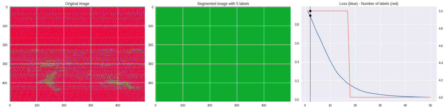
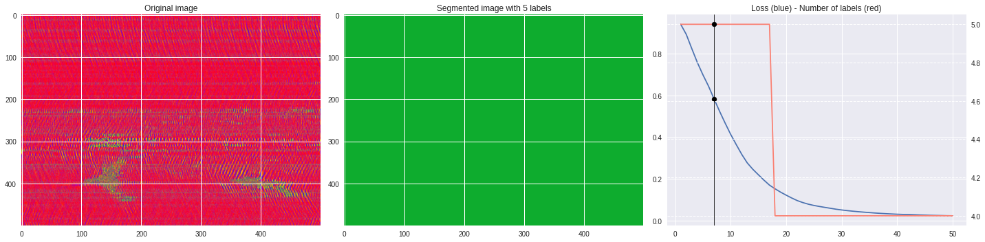
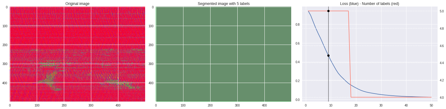
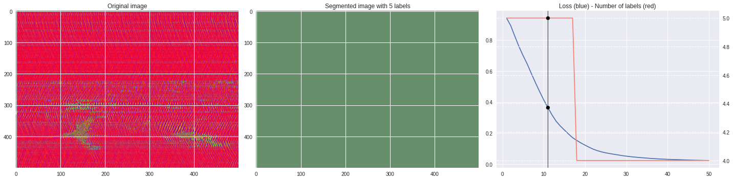
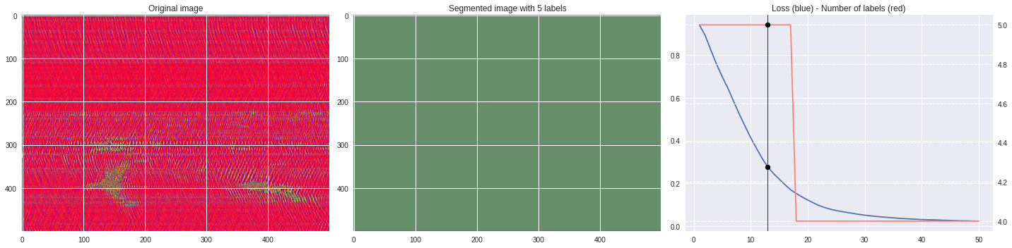
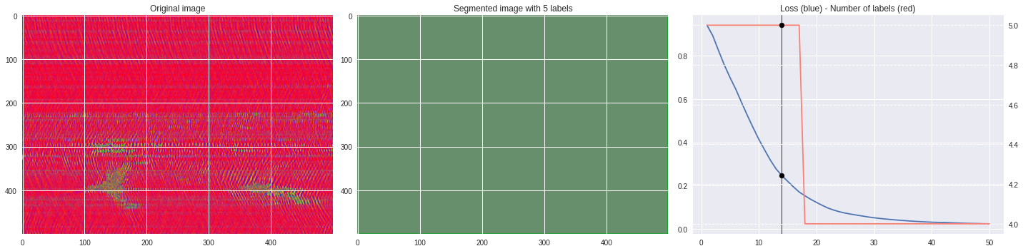
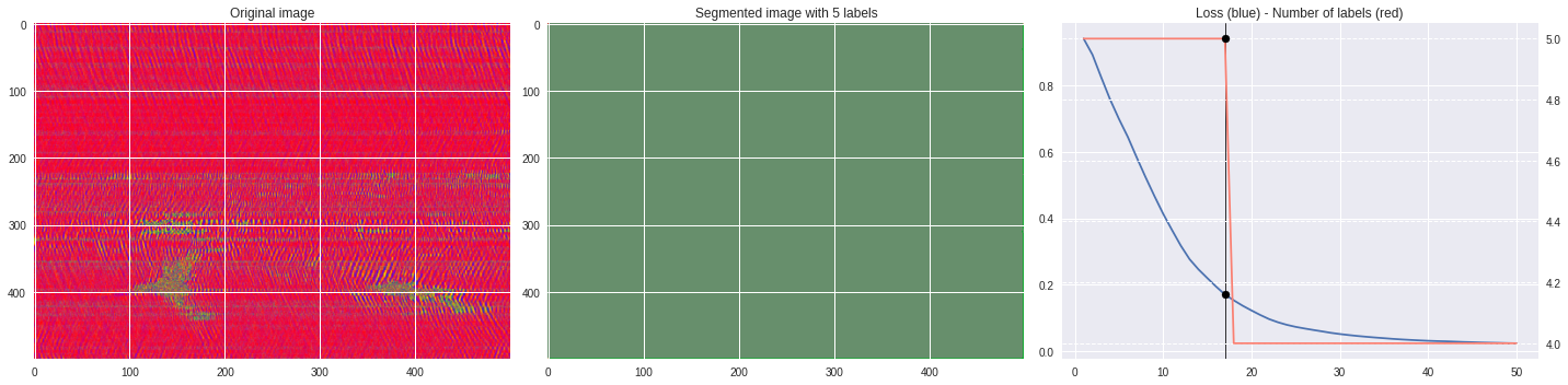
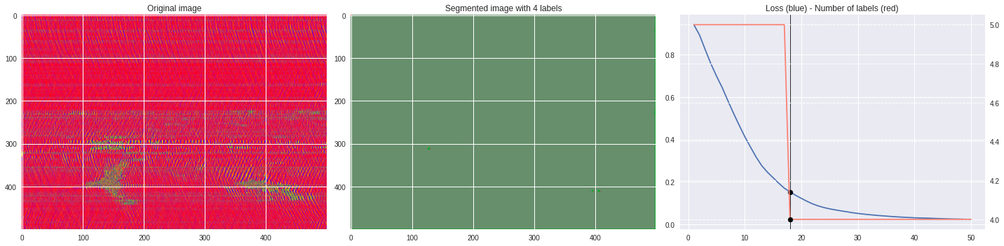
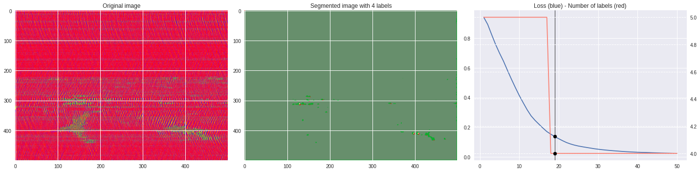
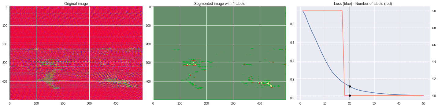
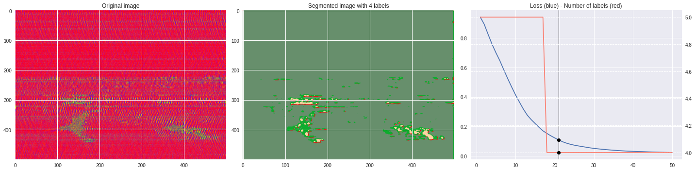
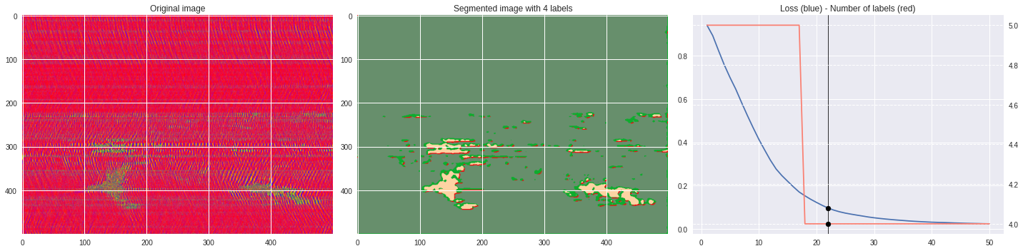
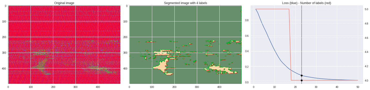
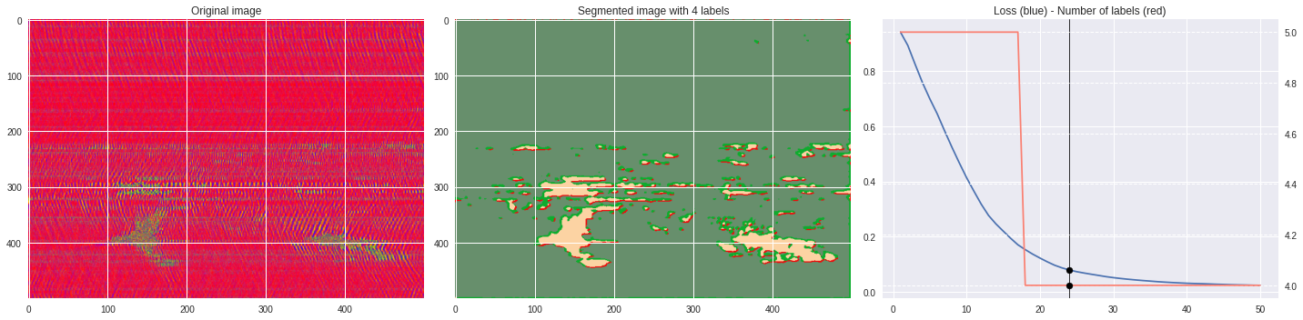
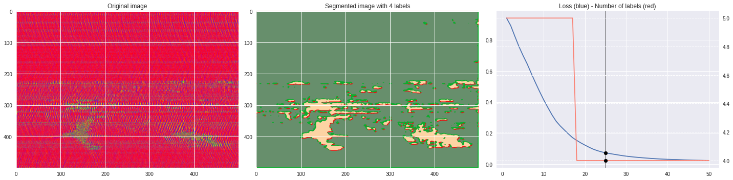
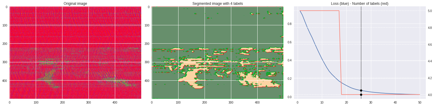
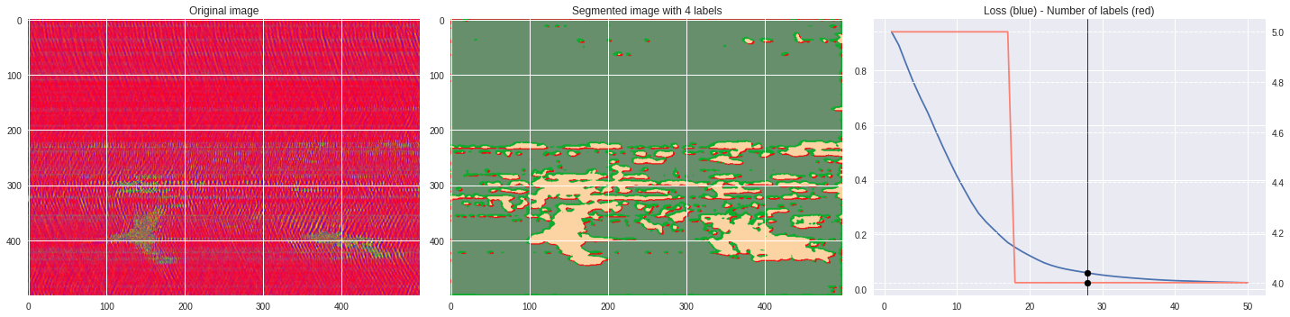
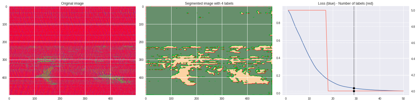
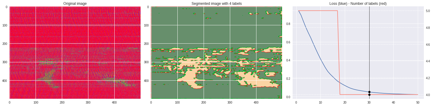
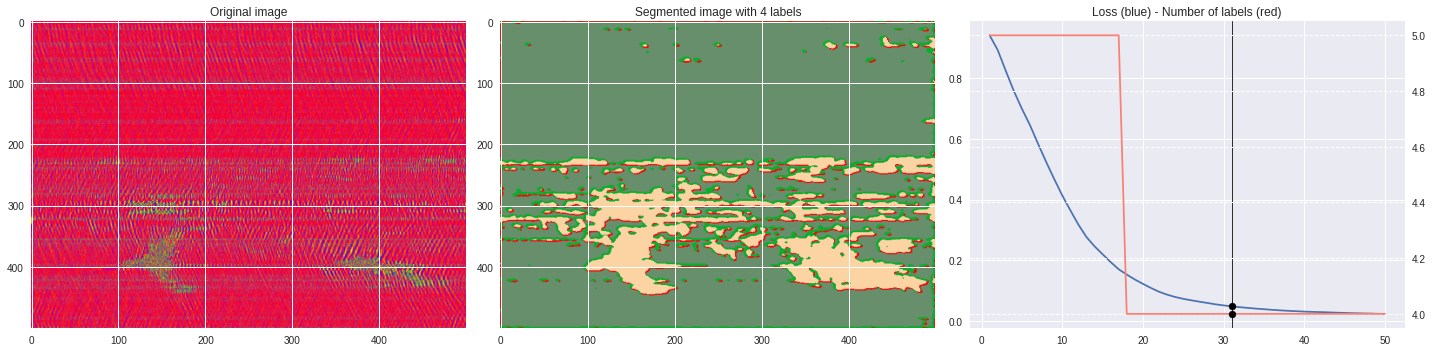
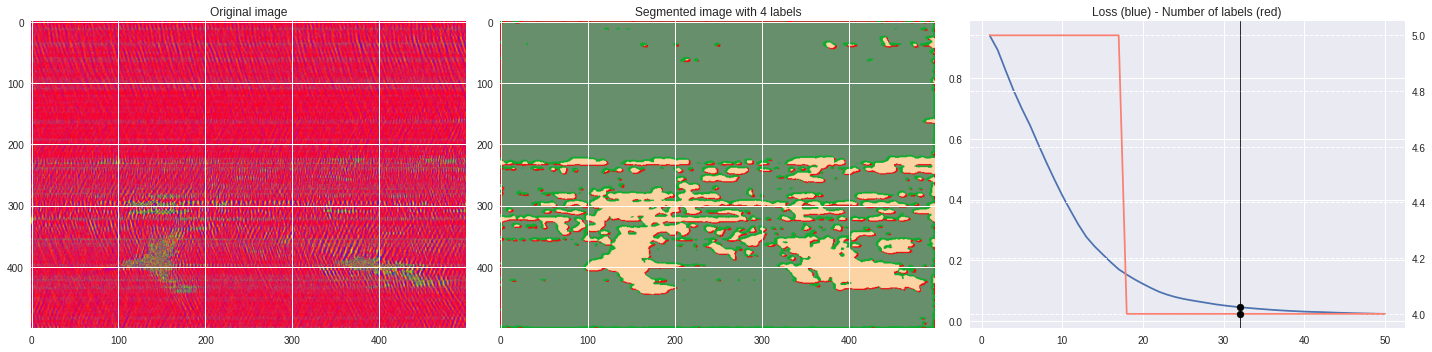
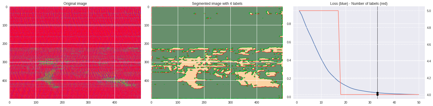
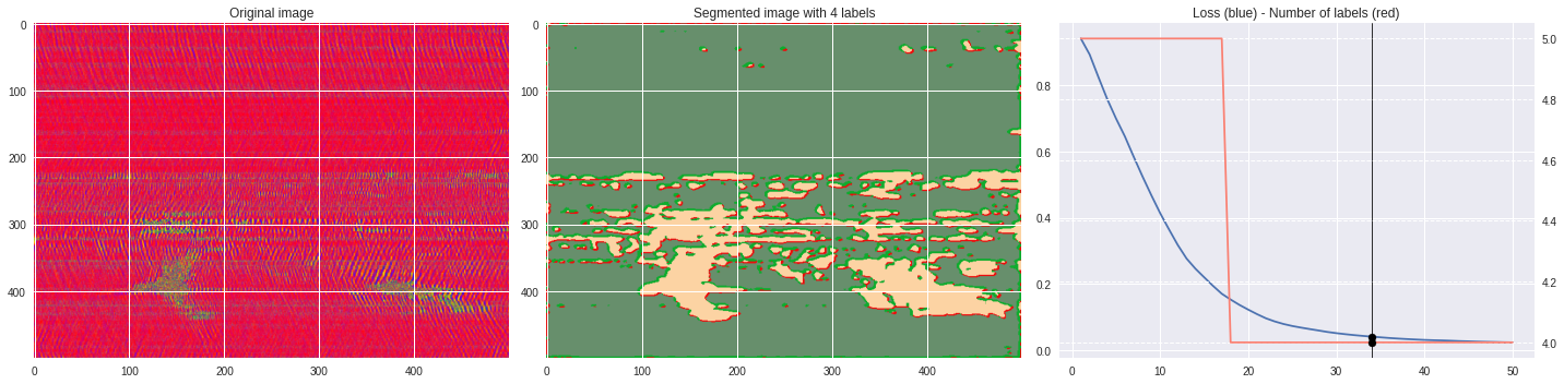
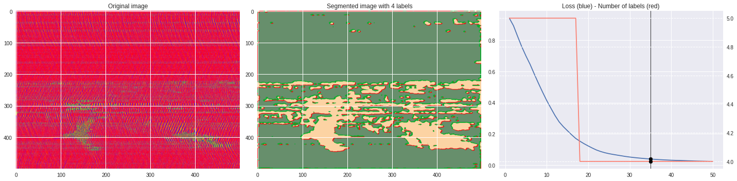
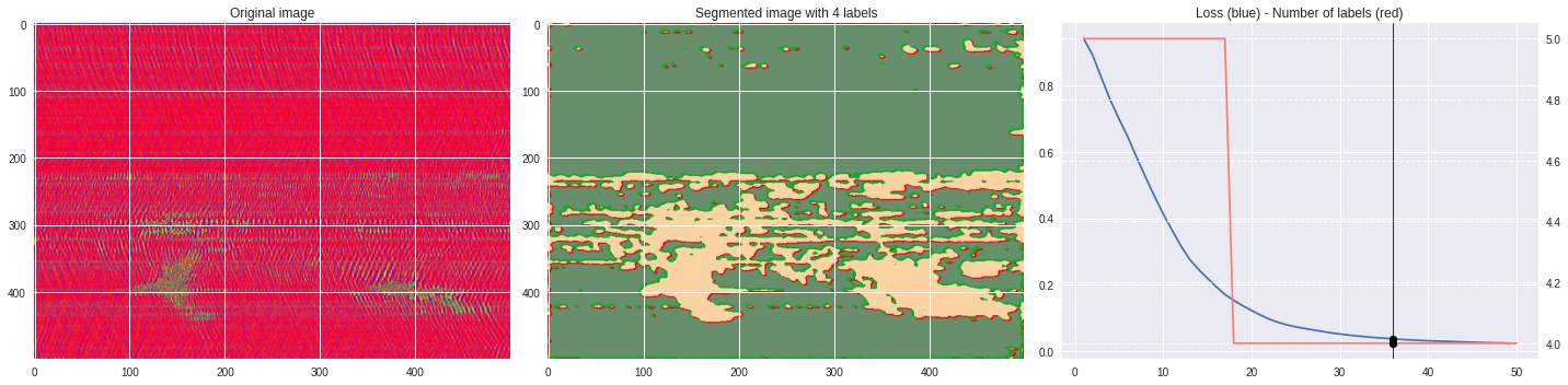
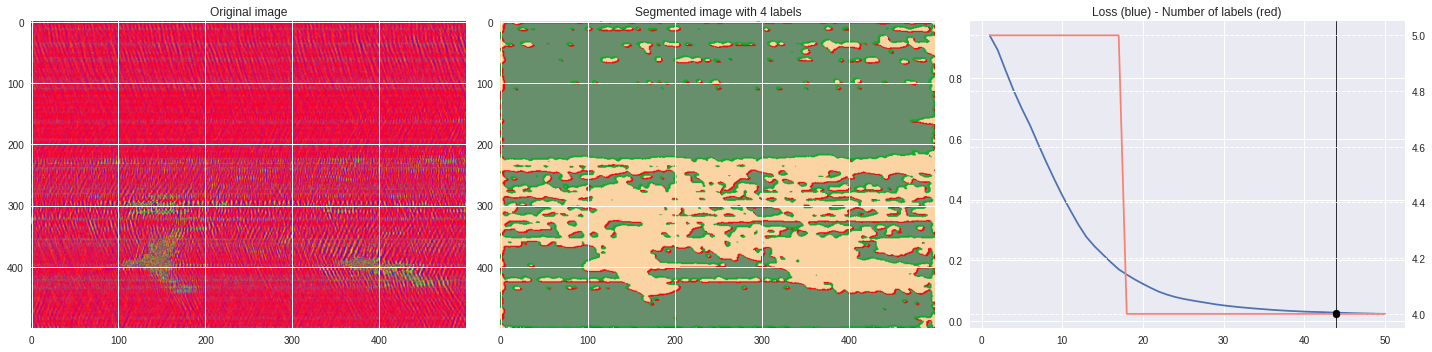
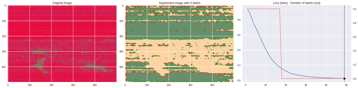
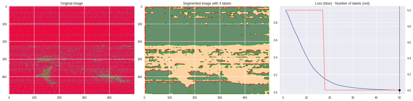
def make_video(im,losses):
  ![ -f video.mp4 ] && rm video.mp4
  losses = numpy.loadtxt(losses)
  for n,loss,nlabels in losses:
    plt.style.use('seaborn')
    fig, (ax1,ax2,ax3) = plt.subplots(1,3,figsize=(20,5))
    ax1.imshow(numpy.squeeze(im),aspect='auto')
    ax1.set_title('Original image')
    ax2.imshow(Image.open('im%03i.png'%n),aspect='auto')
    ax2.set_title('Segmented image with %i labels'%nlabels)
    ax3.plot(losses[:,0],losses[:,1])
    ax3.axvline(n,color='black',lw=0.8,zorder=10)
    ax3.scatter([n],[loss],color='black',zorder=10)
    ax3.set_title('Loss (blue) - Number of labels (red)')
    ax4 = ax3.twinx()
    ax4.grid(ls='dashed')
    ax4.plot(losses[:,0],losses[:,2],color='salmon')
    ax4.scatter([n],[nlabels],color='black',zorder=10)
    plt.tight_layout()
    plt.savefig('im%03i.png'%n)
  !ffmpeg -i im%03d.png video.mp4 && rm im*.png

            

Test on template image ¶

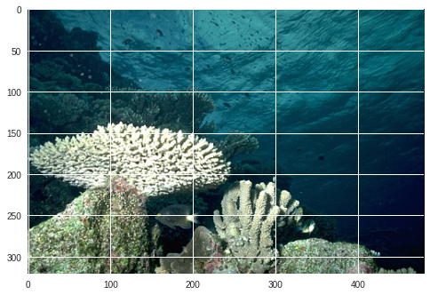
Coral picture ¶

[6]:

             !wget -nv https://raw.githubusercontent.com/kanezaki/pytorch-unsupervised-segmentation/master/images/101027.jpg -O sea.png

            

2020-09-06 16:00:09 URL:https://raw.githubusercontent.com/kanezaki/pytorch-unsupervised-segmentation/master/images/101027.jpg [86536/86536] -> "sea.png" [1]

[14]:

             import numpy
import matplotlib.pyplot as plt
from PIL import Image
im = numpy.array(Image.open('./sea.png'))
print(im.shape)
plt.imshow(im)
plt.show()

            

(321, 481, 3)

../_images/segmentation_segment_36_1.png

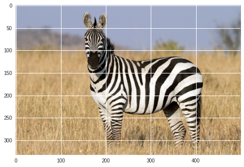
Zebra picture ¶

[ ]:

             !wget -nv https://cdn.mos.cms.futurecdn.net/HjFE8NKWuCmgfHCcndJ3rK.jpg -O zebra.png

            

2020-09-05 05:42:07 URL:https://cdn.mos.cms.futurecdn.net/HjFE8NKWuCmgfHCcndJ3rK.jpg [819084/819084] -> "zebra.png" [1]

[ ]:

             import numpy
from PIL import Image
im = Image.open('./zebra.png')
im = numpy.array(im.resize((500, 333)))
print(im.shape)
plt.imshow(im)
plt.show()

            

(333, 500, 3)

../_images/segmentation_segment_48_1.png

[ ]:

             %%capture
args.maxIter = 20
CNN_seg_train(im,refine=True)
make_video(im,'losses.txt')

            

[ ]:

             mp4 = open('video.mp4','rb').read()
data_url = "data:video/mp4;base64," + b64encode(mp4).decode()
HTML("""<video width=100%% controls loop><source src="%s" type="video/mp4"></video>""" % data_url)

            

Test on DAS data ¶

[75]:

            import h5py,numpy
f = h5py.File('/content/drive/Shared drives/ML4DAS/RawData/30min_files_NoTrain/Dsi_30min_170803000007_170803003007_ch5500_6000.mat','r')
raw = numpy.array(f[f.get('data/dat')[0,0]][:500,:5000])
# f = h5py.File('/content/drive/Shared drives/ML4DAS/RawData/30min_files_Train/Dsi_30min_170730023007_170730030007_ch5500_6000_NS.mat','r')
# raw = numpy.array(f[f.get('dsi30/dat')[0,0]][:500,:5000])
# f = h5py.File('/content/drive/Shared drives/ML4DAS/RawData/1min_ch4650_4850/westSac_180112235958_ch4650_4850.mat','r')
# raw = numpy.array(f[f.get('variable/dat')[0,0]][:500,:5000])

           

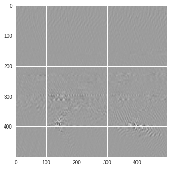
Black and white images ¶

Grayscale images can be used as a first test. Since the data is saved as a 1-channel image, the original numpy array only has 2 dimensions, one for the height (number of rows) and a second for the width (numer of columns). In order for the image segmentation algorithms to work, we reshape the numpy array to include a third dimension specifying the single channel format. We also note that when using the .size attribute on a PIL image, this will return first the width and then the height of the array. Since a numpy array displays the shape in reverse, we reverse the attribute’s returned value so as to not mess up the image.

[ ]:

             import matplotlib.pyplot as plt
from PIL import Image
im = (raw-raw.min())/(raw.max()-raw.min())
im = Image.fromarray(numpy.uint8(im*255)).resize((500, 500))
im = numpy.array(im).reshape(500,500,1)
print(im.shape)
plt.style.use('seaborn')
plt.imshow(im[:,:,0])
plt.show()

            

(500, 500, 1)

../_images/segmentation_segment_55_1.png

[ ]:

             %%capture
args.maxIter = 50
CNN_seg_train(im,refine=True)
make_video(im,'losses.txt')

            

[ ]:

             mp4 = open('video.mp4','rb').read()
data_url = "data:video/mp4;base64," + b64encode(mp4).decode()
HTML("""<video width=100%% controls loop><source src="%s" type="video/mp4"></video>""" % data_url)

            

Colored image ¶

[85]:

             import matplotlib.pyplot as plt
from matplotlib import cm
from PIL import Image
im = (raw-raw.min())/(raw.max()-raw.min())
im = Image.fromarray(numpy.uint8(cm.prism(im)*255)).convert('RGB')
im = numpy.array(im.resize((500, 500)))
labels = segmentation.slic(im, compactness=5, n_segments=4)
print(im.shape)
plt.style.use('seaborn')
plt.imshow(im)
plt.contour(labels,colors='white',linewidths=2)
plt.show()

            

(500, 500, 3)

/usr/local/lib/python3.6/dist-packages/ipykernel_launcher.py:11: UserWarning: No contour levels were found within the data range.
  # This is added back by InteractiveShellApp.init_path()

../_images/segmentation_segment_59_2.png

[92]:

             %%capture
args.maxIter = 50
args.nChannel = 5
args.nConv = 10
args.num_superpixels = 10000
args.compactness = 100
CNN_seg_train(im,refine=False)
make_video(im,'losses.txt')

            

[93]:

             mp4 = open('video.mp4','rb').read()
data_url = "data:video/mp4;base64," + b64encode(mp4).decode()
HTML("""<video width=100%% controls loop><source src="%s" type="video/mp4"></video>""" % data_url)

            

[93]:

Terrain colormap ¶

[ ]:

              mp4 = open('video.mp4','rb').read()
data_url = "data:video/mp4;base64," + b64encode(mp4).decode()
HTML("""<video width=100%% controls loop><source src="%s" type="video/mp4"></video>""" % data_url)

             

[ ]:

              %%capture
args.maxIter = 50
args.nChannel = 100
args.minLabels = 28
CNN_seg_train(im,refine=True)
make_video(im,'losses.txt')

             

[ ]:

              mp4 = open('video.mp4','rb').read()
data_url = "data:video/mp4;base64," + b64encode(mp4).decode()
HTML("""<video width=100%% controls loop><source src="%s" type="video/mp4"></video>""" % data_url)

             

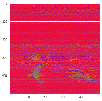
            Prism colormap
            
             ¶
            
              [ ]:

              mp4 = open('video.mp4','rb').read()
data_url = "data:video/mp4;base64," + b64encode(mp4).decode()
HTML("""<video width=100%% controls loop><source src="%s" type="video/mp4"></video>""" % data_url)

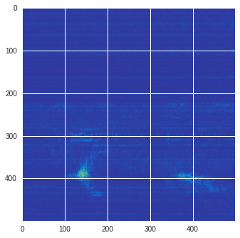
Rescaled amplitude ¶

[137]:

             import matplotlib.pyplot as plt
from matplotlib import cm
from PIL import Image
im = abs(raw)
im = (im-im.min())/(im.max()-im.min())
im = Image.fromarray(numpy.uint8(cm.terrain(im)*255)).convert('RGB')
im = numpy.array(im.resize((500, 500)))
print(im.shape)
plt.style.use('seaborn')
plt.imshow(im)
plt.show()

            

(500, 500, 3)

../_images/segmentation_segment_69_1.png

[ ]:

             %%capture
args.maxIter = 50
CNN_seg_train(im,refine=True)
make_video(im,'losses.txt')

            

[ ]:

             mp4 = open('video.mp4','rb').read()
data_url = "data:video/mp4;base64," + b64encode(mp4).decode()
HTML("""<video width=100%% controls loop><source src="%s" type="video/mp4"></video>""" % data_url)

            

[97]:

             # %%capture
args.maxIter = 50
args.nChannel = 3
args.nConv = 10
args.minLabels = 2
CNN_seg_train(im,refine=False)
# make_video(im,'losses.txt')

            

[98]:

             %%capture
make_video(im,'losses.txt')

[99]:

             mp4 = open('video.mp4','rb').read()
data_url = "data:video/mp4;base64," + b64encode(mp4).decode()
HTML("""<video width=100%% controls loop><source src="%s" type="video/mp4"></video>""" % data_url)

            

[99]:

[100]:

             # %%capture
args.maxIter = 50
args.nChannel = 5
args.nConv = 10
args.minLabels = 3
CNN_seg_train(im,refine=False)
make_video(im,'losses.txt')

            

/usr/local/lib/python3.6/dist-packages/ipykernel_launcher.py:8: RuntimeWarning: More than 20 figures have been opened. Figures created through the pyplot interface (`matplotlib.pyplot.figure`) are retained until explicitly closed and may consume too much memory. (To control this warning, see the rcParam `figure.max_open_warning`).

ffmpeg version 3.4.8-0ubuntu0.2 Copyright (c) 2000-2020 the FFmpeg developers
  built with gcc 7 (Ubuntu 7.5.0-3ubuntu1~18.04)
  configuration: --prefix=/usr --extra-version=0ubuntu0.2 --toolchain=hardened --libdir=/usr/lib/x86_64-linux-gnu --incdir=/usr/include/x86_64-linux-gnu --enable-gpl --disable-stripping --enable-avresample --enable-avisynth --enable-gnutls --enable-ladspa --enable-libass --enable-libbluray --enable-libbs2b --enable-libcaca --enable-libcdio --enable-libflite --enable-libfontconfig --enable-libfreetype --enable-libfribidi --enable-libgme --enable-libgsm --enable-libmp3lame --enable-libmysofa --enable-libopenjpeg --enable-libopenmpt --enable-libopus --enable-libpulse --enable-librubberband --enable-librsvg --enable-libshine --enable-libsnappy --enable-libsoxr --enable-libspeex --enable-libssh --enable-libtheora --enable-libtwolame --enable-libvorbis --enable-libvpx --enable-libwavpack --enable-libwebp --enable-libx265 --enable-libxml2 --enable-libxvid --enable-libzmq --enable-libzvbi --enable-omx --enable-openal --enable-opengl --enable-sdl2 --enable-libdc1394 --enable-libdrm --enable-libiec61883 --enable-chromaprint --enable-frei0r --enable-libopencv --enable-libx264 --enable-shared
  libavutil      55. 78.100 / 55. 78.100
  libavcodec     57.107.100 / 57.107.100
  libavformat    57. 83.100 / 57. 83.100
  libavdevice    57. 10.100 / 57. 10.100
  libavfilter     6.107.100 /  6.107.100
  libavresample   3.  7.  0 /  3.  7.  0
  libswscale      4.  8.100 /  4.  8.100
  libswresample   2.  9.100 /  2.  9.100
  libpostproc    54.  7.100 / 54.  7.100
Input #0, image2, from 'im%03d.png':
  Duration: 00:00:02.00, start: 0.000000, bitrate: N/A
    Stream #0:0: Video: png, rgba(pc), 1440x360 [SAR 2834:2834 DAR 4:1], 25 fps, 25 tbr, 25 tbn, 25 tbc
Stream mapping:
  Stream #0:0 -> #0:0 (png (native) -> h264 (libx264))
Press [q] to stop, [?] for help
[libx264 @ 0x565236e5fe00] using SAR=1/1
[libx264 @ 0x565236e5fe00] using cpu capabilities: MMX2 SSE2Fast SSSE3 SSE4.2 AVX FMA3 BMI2 AVX2 AVX512
[libx264 @ 0x565236e5fe00] profile High 4:4:4 Predictive, level 3.1, 4:4:4 8-bit
[libx264 @ 0x565236e5fe00] 264 - core 152 r2854 e9a5903 - H.264/MPEG-4 AVC codec - Copyleft 2003-2017 - http://www.videolan.org/x264.html - options: cabac=1 ref=3 deblock=1:0:0 analyse=0x1:0x111 me=hex subme=7 psy=1 psy_rd=1.00:0.00 mixed_ref=1 me_range=16 chroma_me=1 trellis=1 8x8dct=0 cqm=0 deadzone=21,11 fast_pskip=1 chroma_qp_offset=4 threads=3 lookahead_threads=1 sliced_threads=0 nr=0 decimate=1 interlaced=0 bluray_compat=0 constrained_intra=0 bframes=3 b_pyramid=2 b_adapt=1 b_bias=0 direct=1 weightb=1 open_gop=0 weightp=2 keyint=250 keyint_min=25 scenecut=40 intra_refresh=0 rc_lookahead=40 rc=crf mbtree=1 crf=23.0 qcomp=0.60 qpmin=0 qpmax=69 qpstep=4 ip_ratio=1.40 aq=1:1.00
Output #0, mp4, to 'video.mp4':
  Metadata:
    encoder         : Lavf57.83.100
    Stream #0:0: Video: h264 (libx264) (avc1 / 0x31637661), yuv444p, 1440x360 [SAR 1:1 DAR 4:1], q=-1--1, 25 fps, 12800 tbn, 25 tbc
    Metadata:
      encoder         : Lavc57.107.100 libx264
    Side data:
      cpb: bitrate max/min/avg: 0/0/0 buffer size: 0 vbv_delay: -1
frame=   50 fps= 34 q=-1.0 Lsize=     317kB time=00:00:01.88 bitrate=1380.9kbits/s speed=1.28x
video:316kB audio:0kB subtitle:0kB other streams:0kB global headers:0kB muxing overhead: 0.419917%
[libx264 @ 0x565236e5fe00] frame I:1     Avg QP:17.61  size: 96131
[libx264 @ 0x565236e5fe00] frame P:27    Avg QP:23.39  size:  5205
[libx264 @ 0x565236e5fe00] frame B:22    Avg QP:30.54  size:  3901
[libx264 @ 0x565236e5fe00] consecutive B-frames: 26.0% 40.0% 18.0% 16.0%
[libx264 @ 0x565236e5fe00] mb I  I16..4: 61.3%  0.0% 38.7%
[libx264 @ 0x565236e5fe00] mb P  I16..4:  2.1%  0.0%  1.9%  P16..4:  3.3%  2.2%  2.1%  0.0%  0.0%    skip:88.4%
[libx264 @ 0x565236e5fe00] mb B  I16..4:  0.4%  0.0%  0.2%  B16..8:  6.6%  3.0%  1.9%  direct: 1.9%  skip:86.1%  L0:55.7% L1:35.9% BI: 8.5%
[libx264 @ 0x565236e5fe00] coded y,u,v intra: 34.0% 25.3% 30.0% inter: 3.0% 0.7% 3.7%
[libx264 @ 0x565236e5fe00] i16 v,h,dc,p: 63% 31%  5%  0%
[libx264 @ 0x565236e5fe00] i4 v,h,dc,ddl,ddr,vr,hd,vl,hu: 26% 33% 16%  3%  3%  6%  4%  4%  4%
[libx264 @ 0x565236e5fe00] Weighted P-Frames: Y:0.0% UV:0.0%
[libx264 @ 0x565236e5fe00] ref P L0: 62.9%  9.8% 16.5% 10.8%
[libx264 @ 0x565236e5fe00] ref B L0: 86.7% 11.2%  2.1%
[libx264 @ 0x565236e5fe00] ref B L1: 98.8%  1.2%
[libx264 @ 0x565236e5fe00] kb/s:1289.88